Spatial Distribution Analysis Methodology for News Image Processing

Overview

Spatial Distribution Analysis is a critical component in converting 2D news images into accurate 3D virtual environments. This methodology examines how objects, people, and features are positioned and distributed across space, providing essential data for realistic virtual reconstruction.

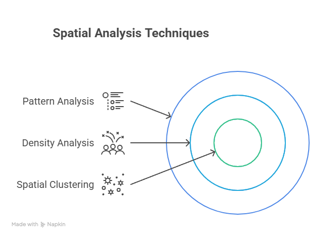
Core Analysis Framework

1. Pattern Analysis: Understanding Spatial Arrangements

Pattern analysis examines the fundamental organization of elements within an image to determine the underlying spatial structure.

1.1 Random Distribution Detection

Definition: Elements scattered without apparent order or systematic arrangement

Identification Criteria:

• No discernible pattern or structure

• Irregular spacing between objects

• Variable distances with no consistent relationships

• Absence of geometric or systematic arrangements

Measurement Methods:

• Nearest Neighbor Analysis: Calculate average distance to closest neighbor

• Quadrat Analysis: Divide image into grid squares and count elements per square

• Variance-to-Mean Ratio: Values near 1.0 indicate random distribution

Algorithm Implementation:

For each object position (x,y): 1. Calculate distance to nearest neighbor 2. Compare with expected random distribution 3. Apply statistical significance tests 4. Generate randomness coefficient (0-1 scale)

1.2 Regular (Even) Distribution Analysis

Definition: Elements arranged in systematic, predictable patterns with consistent spacing

Identification Markers:

• Uniform spacing between similar objects

• Geometric patterns (grid, linear, radial)

• Consistent angular relationships

• Repetitive structural arrangements

Detection Techniques:

• Grid Detection Algorithm: Identify regular spacing intervals

• Fourier Transform Analysis: Detect periodic patterns in spatial frequencies

• Template Matching: Compare against known regular patterns

Measurement Parameters:

• Spacing uniformity coefficient

• Pattern deviation metrics

• Geometric alignment scores

• Regularity index (0-1 scale)

1.3 Clustered (Grouped) Distribution Identification

Definition: Elements gathered in distinct groups with higher internal density than external spacing

Clustering Characteristics:

• High concentration of elements in specific areas

• Clear separation between groups

• Variable cluster sizes and densities

• Empty or sparse areas between clusters

Analysis Process:

1. Distance Matrix Calculation → Compute all pairwise distances between objects 2. Cluster Boundary Detection → Apply distance thresholds to identify groups 3. Cluster Validation → Verify statistical significance of groupings 4. Cluster Characterization → Measure size, density, and separation metrics

2. Density Analysis: Quantifying Spatial Concentration

2.1 High-Density Zone Detection

Objective: Identify areas with concentrated elements requiring detailed 3D modeling

Methodology:

Step 1: Grid-Based Density Mapping

• Divide image into uniform grid cells

• Count elements per cell

• Calculate density ratios

• Generate heat map visualization

Step 2: Kernel Density Estimation

• Apply Gaussian kernels around each object

• Sum overlapping kernels to create smooth density surface

• Identify peak density regions

• Calculate confidence intervals

Step 3: Threshold-Based Classification

Density Categories: - Ultra-High: > 95th percentile - High: 75th-95th percentile - Medium: 25th-75th percentile - Low: < 25th percentile

Applications:

• Crowd concentration analysis

• Vehicle traffic density

• Building concentration mapping

• Urban development patterns

2.2 Low-Density and Scattered Zone Analysis

Purpose: Identify sparse areas and understand negative space in 3D reconstruction

Detection Methods:

Voronoi Diagram Analysis:

• Generate Voronoi cells around each object

• Large cells indicate low-density areas

• Calculate area-to-object ratios

• Identify isolation patterns

Distance-Based Metrics:

• Mean nearest neighbor distance

• Standard deviation of spacing

• Isolation index calculation

• Connectivity measurements

Empty Space Identification:

• Binary image processing to find object-free areas

• Connected component analysis for continuous empty regions

• Morphological operations to clean noise

• Area calculation for significant empty zones

3. Spatial Clustering Algorithms for Feature Detection

3.1 K-Means Clustering Implementation

Algorithm Overview: Partitions data points into k clusters based on spatial proximity

Process Flow:

1. Initialization → Select k initial cluster centers → Define distance metric (Euclidean, Manhattan) 2. Assignment Phase → Assign each object to nearest cluster center → Calculate membership matrices 3. Update Phase → Recalculate cluster centers as centroids → Update positions based on member coordinates 4. Convergence Check → Compare new centers with previous positions → Stop when movement < threshold or max iterations reached 5. Validation → Calculate within-cluster sum of squares (WCSS) → Assess cluster quality metrics

Parameter Selection:

• Optimal k Selection: Elbow method, silhouette analysis

• Distance Metrics: Euclidean for geometric clustering, Manhattan for grid-based

• Convergence Criteria: Position tolerance, iteration limits

Applications in News Image Analysis:

• Grouping people in crowd scenes

• Organizing vehicle clusters in traffic

• Categorizing building groups by type or size

3.2 DBSCAN (Density-Based Spatial Clustering) Method

Algorithm Advantages: Automatically determines cluster count and handles irregular shapes

Core Parameters:

• Epsilon (ε): Maximum distance between points in same neighborhood

• MinPts: Minimum number of points required to form dense region

Implementation Steps:

1. Neighborhood Definition → For each point, find all points within ε distance → Create neighborhood lists 2. Core Point Identification → Mark points with ≥ MinPts neighbors as core points → Identify border and noise points 3. Cluster Formation → Start with unvisited core point → Add all density-reachable points to cluster → Repeat until all core points processed 4. Result Classification → Core points: cluster members → Border points: edge of clusters → Noise points: outliers or isolated elements

Advantages for Spatial Analysis:

• No need to specify cluster count in advance

• Handles clusters of arbitrary shapes

• Identifies outliers and noise points

• Robust to varying densities

3.3 Vegetation Detection Case Study

Objective: Identify and map plant/vegetation areas using spatial clustering

Multi-Step Approach:

Step 1: Color-Based Pre-filtering

• Convert image to HSV color space

• Define green color ranges for vegetation

• Create binary mask for potential vegetation pixels

• Apply morphological operations to reduce noise

Step 2: Spatial Clustering Application

DBSCAN Parameters for Vegetation: - ε = 5-10 pixels (based on image resolution) - MinPts = 20-50 points (ensures significant vegetation areas) - Distance metric = Euclidean in 2D pixel coordinates

Step 3: Cluster Validation and Refinement

• Filter clusters by minimum area thresholds

• Analyze cluster shape properties (compactness, elongation)

• Cross-validate with texture analysis

• Remove false positives (green objects that aren't vegetation)

Step 4: Vegetation Zone Classification

Cluster Categories: - Dense Forest: Large, compact clusters (>1000 pixels) - Scattered Trees: Small, isolated clusters (50-200 pixels) - Grass Areas: Elongated, low-density clusters - Mixed Vegetation: Irregular, moderate-density clusters

Quality Metrics and Validation

Statistical Measures

• Silhouette Coefficient: Cluster quality assessment (-1 to +1)

• Calinski-Harabasz Index: Ratio of between-cluster to within-cluster variance

• Davies-Bouldin Index: Average similarity between clusters

Spatial Validation

• Hopkins Statistic: Test for spatial randomness

• Moran's I: Measure of spatial autocorrelation

• Getis-Ord G: Local clustering significance test

Integration with 3D Reconstruction

Data Output Format

• Cluster membership matrices

• Density heat maps

• Pattern classification labels

• Spatial relationship graphs

3D Modeling Applications

• Object placement algorithms use clustering results

• Density maps inform level-of-detail (LOD) strategies

• Pattern analysis guides procedural generation

• Spatial relationships maintain realistic positioning

Conclusion

Spatial Distribution Analysis provides the foundational spatial intelligence necessary for accurate 3D reconstruction of news images. By systematically analyzing patterns, densities, and spatial relationships, this methodology ensures that virtual environments maintain the authentic spatial characteristics of the original scenes, creating more immersive and realistic simulations for educational, research, and analytical purposes.